Blog

How to Create Company and Ledger in Tally Prime: Complete Step-by-Step Guide

Tally Prime is one of the most trusted accounting and GST compliance software used by millions of businesses. Whether you are a beginner in accounting or a professional managing multiple clients, knowing how to create a Company and Ledgers in Tally Prime is essential. Without proper company setup and ledger creation, no business transactions can be recorded accurately.

In this detailed guide, you will learn what a company in Tally means, how to create one, how to configure its features, how to create essential ledgers, and how to organize your chart of accounts effectively. This article is written in a simple and practical manner with tables, tips, and examples for better understanding.

What Is a Company in Tally Prime?

A Company in Tally Prime represents the business entity whose books of accounts you want to maintain. It contains essential information such as:

Company Name
Financial Year
Books Beginning Date
Address and Contact Details
GST Information
Currency Details
Security Controls
Financial and Accounting Preferences

Tally Prime allows unlimited companies to be created and maintained in a single system. They can be opened, shut, altered, backed up, and restored anytime.

How to Create a Company in Tally Prime

You can create a company in Tally Prime through the Create Company menu.

Step-by-Step Process

Step 1: Open Tally Prime

Start Tally Prime from your desktop.
Once it opens, you will see the Gateway of Tally screen.

Step 2: Go to Create Company

You will see the following options:

Create Company
Select Company
Shut Company

Choose Create Company.

Step 3: Enter Company Details

Fill in the details as required.

Field	Description
Directory	Where your company data will be stored
Name	Official name of your business
Mailing Name	Name to print on invoices
Address	Company address
Country	Location of business
State	State for GST applicability
Pincode	Postal code
Phone/Email	Contact information
Financial Year Begin	Start of financial year, e.g., 01-04-2024
Books Begin From	Start date of accounts
Currency	Auto-filled based on country

Step 4: Enable GST and Other Features

After entering basic details, enable additional features as needed:

Enable GST
Maintain Accounts with Inventory
Enable Security Control
Enable TDS/TCS
Enable Payroll

Each business requires different modules depending on operations.

Step 5: Save the Company

Press Ctrl + A to save the company.
Now your Tally company is successfully created.

Additional Company Configurations

Once created, you can configure additional settings through:
Gateway of Tally > F11 (Features)

Some commonly used configurations are:

Feature	Purpose
Accounting Features	Enable credit limits, bill-wise details, cost centers
Inventory Features	Enable batches, expiry dates, godowns
Statutory Features	Enable GST, TDS, TCS, PF, ESI
Invoice Features	Enable item-wise tax, discount, e-way bill options

These settings help customize Tally Prime based on your business needs.

What Is a Ledger in Tally Prime?

A Ledger is an accounting head under which financial transactions are recorded.
Tally uses a group and ledger system based on the accounting hierarchy.

Examples of commonly used ledgers:

Cash
Bank Accounts
Sundry Debtors
Sundry Creditors
Purchase
Sales
Duties & Taxes
Capital Account
Fixed Assets
Expenses (Direct & Indirect)

A company must have at least two ledgers to start:

Cash
Profit & Loss A/c (Created automatically)

All other ledgers must be created manually.

How to Create a Ledger in Tally Prime

Step-by-Step Process for Creating a Ledger

Step 1: Go to Ledger Creation Screen

Gateway of Tally > Create > Ledger
OR
Press Alt + C while entering a voucher.

Step 2: Enter Ledger Details

Fill in the required details.

Field	Description
Name	Ledger name (e.g., ABC Traders)
Group	Correct group classification such as Sundry Debtors
Opening Balance	Opening value if any
GST Details	For GST registered ledgers
Mailing Details	For customers and suppliers

Step 3: Group Selection

Selecting the right group is very important because it affects:

Financial statements
Trial balance
Profit and loss
Balance sheet classification

Example:
Sale ledger should be under Sales Accounts,
Supplier ledger under Sundry Creditors,
Customer ledger under Sundry Debtors,
Expenses under Indirect Expenses.

Step 4: Save Ledger

Press Ctrl + A to save.

Types of Ledgers You Should Create in Every New Company

Below is a practical list of common ledgers used in most businesses:

1. Capital and Owner-Related Ledgers

Capital Account
Drawings

2. Banking Ledgers

Bank Account Name
Bank OD/CC Accounts

3. Sales and Purchase Ledgers

Sales GST 5 percent
Sales GST 12 percent
Sales GST 18 percent
Purchase GST 5 percent
Purchase GST 12 percent
Purchase GST 18 percent

4. Tax Ledgers

CGST
SGST
IGST
TDS Payable
TCS Payable

5. Customer and Supplier Ledgers

Each customer and supplier has its individual ledger.

6. Expense Ledgers

Rent
Salary
Office Expenses
Electricity Expenses
Telephone Charges
Stationery

7. Asset and Liability Ledgers

Furniture
Computers
Building
Loan Accounts
Outstanding Expenses

Example Table: Ledger and Its Group

Ledger Name	Group
ABC Traders	Sundry Debtors
Rent Expense	Indirect Expenses
CGST Payable	Duties & Taxes
SBI Bank A/c	Bank Accounts

Important Tips for Creating Accurate Ledgers in Tally Prime

Here are must-follow guidelines to avoid errors:

1. Use Proper Naming Conventions

Examples:

Don’t use abbreviations without clarity.
Use customer/supplier names exactly as per invoices.

2. Select Correct Group Always

Grouping mistakes can cause wrong balance sheet or P&L results.

3. Maintain Opening Balances Carefully

Incorrect opening balances can reflect wrong totals throughout the year.

4. Enable Bill-Wise Details

Useful for tracking customer invoices, outstanding payments, and supplier credits.

5. Add GST Details for Taxable Ledgers

For customers and suppliers:

GSTIN
Registration type
State
Tax applicability

For product-based ledgers:

GST rate
HSN/SAC code

6. Use Mailing Details for Parties

This helps generate invoices, statements, and reports accurately.

7. Regularly Review the Chart of Accounts

Tally Prime allows viewing all ledgers through:
Gateway of Tally > Chart of Accounts

This helps identify:

Duplicate ledgers
Wrong groups
Incomplete details

Example: Creating a Customer Ledger

To create a ledger for a customer named Sharma Traders:

Name: Sharma Traders
Group: Sundry Debtors
Maintain balances: Yes
Enable bill-wise details: Yes
Opening balance: Enter outstanding receivable
GSTIN: If available
State: Required for intra-state or inter-state supply

This ensures proper tracking of sales, receipts, and outstanding balances.

Example: Creating a Sales Ledger with GST

For GST-based sales at 18 percent:

Name: Sales 18 Percent
Group: Sales Accounts
Type of supply: Goods or Services
GST Rate: 18 percent
HSN/SAC: Enter if known

This ledger will automatically calculate GST in invoices.

Conclusion

Creating a Company and Ledger in Tally Prime is the foundation of maintaining accurate and compliant accounts. With proper setup, correct grouping, and well-structured ledgers, your accounting process becomes smooth and error-free. This guide explained company creation, ledger creation, essential fields, GST setups, grouping, and best practices in a simple and comprehensive format. Whether you are running a small business or managing large-scale operations, mastering these basics will significantly improve your accounting efficiency.

Disclaimer

This article is intended for educational purposes. Tally Prime features may vary depending on updates and configurations. Users should apply settings based on their business requirements.

December 4, 2025

How to Use VLOOKUP with IFERROR in Excel for Clean, Error-Free Data Lookup: Complete Step-by-Step Guide

VLOOKUP is one of the most widely used lookup functions in Excel, but it often returns annoying errors like #N/A whenever a match is not found. These errors can make your reports look unprofessional and can even break dependent formulas. By combining VLOOKUP with IFERROR, you can control the output, replace errors with meaningful messages, and create more polished dashboards and reports.

In this in-depth guide, you will learn how VLOOKUP works, why IFERROR is necessary, practical examples, best practices, and advanced usage tips. This tutorial is designed to be simple, clear, and ideal for beginners as well as advanced Excel users who want clean, reliable lookup results.

What Is VLOOKUP?

VLOOKUP (Vertical Lookup) searches for a value in the leftmost column of a table and returns a matching value from a column to the right of it.

Basic VLOOKUP syntax:
=VLOOKUP(lookup_value, table_array, col_index_num, [range_lookup])

Explanation in simple terms:

Part	Meaning
lookup_value	The value you want to search
table_array	The table from which you want data
col_index_num	The column number from where result is fetched
range_lookup	TRUE for approximate match, FALSE for exact match

Although VLOOKUP is powerful, it has one drawback: it shows errors when a match is not found. This is where IFERROR becomes extremely useful.

Why Add IFERROR to VLOOKUP?

IFERROR is used to catch any error in a formula and return an alternative value.

IFERROR syntax:
=IFERROR(value, value_if_error)

This means:

If a formula works, show the result.
If it fails, show your custom message instead of an error.

Common scenarios where VLOOKUP returns errors:

Item not found in the list
Extra spaces in lookup values
Wrong column number
Missing data
Typing mistakes in lookup value

By wrapping VLOOKUP with IFERROR, you ensure clean and user-friendly results.

Basic Formula: VLOOKUP with IFERROR

The most commonly used format:

=IFERROR(VLOOKUP(A2, D2:E20, 2, FALSE), "Not Found")

This formula means:

Search value in A2 within the range D2:E20
If a match exists, return column 2
If not, return the message “Not Found”

You can replace “Not Found” with:

0
Blank (“”)
Custom text, like “No Record”

Practical Example: Product Price Lookup

Suppose you have a product list with two columns: Product Code and Price.

Product Code	Price
P101	250
P102	300
P103	450
P104	520

Now you want to look up the price of a product entered by the user.

Let’s say the lookup value is in B2.
Normal VLOOKUP:
=VLOOKUP(B2, A2:B5, 2, FALSE)

If the product code doesn’t exist, Excel will show #N/A.

Error-free version:
=IFERROR(VLOOKUP(B2, A2:B5, 2, FALSE), "Price Not Available")

This makes your sheet look professional and avoids confusion for your end user.

Common Real-Life Use Cases

1. Employee Salary Lookup

In companies, VLOOKUP is often used to fetch salaries by employee ID.
If the ID is not found or wrongly typed, showing a message like “Invalid ID” makes more sense.

Formula:
=IFERROR(VLOOKUP(E2, A2:C500, 3, FALSE), "Invalid ID")

2. Student Marks Retrieval

Schools use VLOOKUP to match student roll numbers with their marks.
Errors can cause unnecessary panic; IFERROR prevents this.

Formula:
=IFERROR(VLOOKUP(A2, G2:J200, 4, FALSE), "No Marks Available")

3. Customer Data Lookup in CRM

CRM users often search customer names or ID numbers.
Returning a clean message helps avoid confusion when data is missing.

Best Practices When Using VLOOKUP with IFERROR

Tip	Benefit
Always use FALSE for exact match	Prevents wrong results
Clean spaces using TRIM	Avoids lookup mismatches
Lock ranges with $ sign	Safe copy-paste across sheet
Return blank instead of message	Cleaner dashboards
Use IFERROR only at final output	Improves performance

Advanced Ways to Use IFERROR with VLOOKUP

1. VLOOKUP + IFERROR + TRIM

Useful when text contains extra spaces.

=IFERROR(VLOOKUP(TRIM(A2), D2:E100, 2, FALSE), "Not Found")

2. Return Blank Instead of Text

For dashboards or MIS reports:

=IFERROR(VLOOKUP(A2, D2:E100, 2, FALSE), "")

3. Nesting Multiple VLOOKUPs

When searching in multiple lists:

=IFERROR(VLOOKUP(A2, Data1, 2, FALSE), IFERROR(VLOOKUP(A2, Data2, 2, FALSE), "No Match"))

4. VLOOKUP with IFERROR for Approximate Match

For commission slabs, rate charts, GST slabs:

=IFERROR(VLOOKUP(A2, D2:E10, 2, TRUE), 0)

Performance Tips When Using IFERROR

Although IFERROR is highly helpful, overusing it can slow down large Excel files, especially when thousands of rows are involved.

Key performance points:

Evaluate the formula logic first—only wrap final formula with IFERROR.
Avoid using IFERROR inside array formulas unless required.
If performance becomes an issue, switch to INDEX + MATCH (faster in many cases).
Use Excel Tables so that VLOOKUP uses structured references (improves clarity and reduces errors).
Avoid volatile functions with VLOOKUP, such as INDIRECT or OFFSET unnecessarily.

Example Table: Comparing VLOOKUP vs VLOOKUP + IFERROR

Function	Outcome
VLOOKUP only	Shows #N/A for no match
VLOOKUP + IFERROR	Shows clean custom output

When Should You Avoid IFERROR?

Although powerful, IFERROR hides all errors, not just #N/A.
This may hide genuine issues like:

Wrong range selected
Incorrect column index
Missing data
Unintended empty columns

If you need to handle only #N/A, use IFNA instead:
=IFNA(VLOOKUP(A2, D2:E20, 2, FALSE), "Not Found")

Final Example: Clean Lookup Template Formula

Here is a complete, optimized formula used in many professional MIS reports:

=IFERROR(VLOOKUP(TRIM(A2), $D$2:$E$500, 2, FALSE), "")

This ensures:

Leading/trailing spaces removed
Fixed lookup range
Exact match
Clean blank output

Conclusion

Using VLOOKUP with IFERROR is essential for creating clean, error-free, and user-friendly Excel reports. Whether you are working on employee databases, inventory lists, student marksheets, or detailed MIS dashboards, this combination ensures polished results without confusing error messages. With the examples and tips provided above, you can confidently apply this formula in real projects and maintain a professional standard in your Excel work.

Disclaimer

This article is for educational and informational purposes only. Excel functions and features may vary based on version and updates. Users should verify results based on their specific data structure.

December 4, 2025

How to Prepare GST Summary Report in Excel: A Complete Step-by-Step Guide for Businesses

Preparing a detailed and accurate GST Summary Report in Excel is essential for GST return filing, internal control, sales analysis, purchase analytics, input tax credit (ITC) tracking, and audit readiness. Whether a business files monthly GSTR-3B or quarterly returns, a GST summary prepared in Excel ensures that every taxable value, rate-wise bifurcation, and tax amount is verified before uploading to the GST portal.

Excel is the easiest and most flexible tool for preparing GST reports because it allows customized formulas such as SUMIF, SUMIFS, VLOOKUP, INDEX MATCH, Pivot Tables, and Conditional Formatting. In this guide, you will learn how to prepare a professional GST Summary Report in Excel from raw sales and purchase data.

1. Understanding GST Summary Report

A GST Summary Report is a consolidated statement that summarises business transactions under GST for a specific period, usually monthly or quarterly. It includes total outward supplies, inward supplies, taxable value, tax rate, CGST, SGST, IGST, exempt supplies, and ITC.

Typical values included:

Total Sales
B2B Sales
B2C Sales
Zero Rated Supplies
Nil/Exempt Supply
Total Purchases
Input Tax Credit (ITC) Availed
RCM Liability
Net Payable

2. Data Required to Prepare GST Summary in Excel

To prepare the GST report, you need:

Detailed Sales Register
Detailed Purchase Register
Debit Notes and Credit Notes
Expenses on which RCM is applicable
Opening and Closing ITC values (if needed)

A typical sales or purchase register contains:

Invoice Number
Invoice Date
Customer / Supplier Name
GSTIN
Place of Supply
Taxable Value
GST Rate
CGST, SGST, IGST Amount
Total Invoice Amount

With this data, we can prepare the summary.

3. Formatting Data to Create GST Summary Report

The first and most important step is cleaning the raw data. GST data often contains duplicates, wrong tax calculations, missing GSTINs, and unclassified transactions, so formatting is necessary.

Important Formatting Steps

Convert data into Excel Table (Ctrl + T).
Ensure dates are correct using proper date format.
Verify GST rates: 0%, 5%, 12%, 18%, 28%.
Apply Conditional Formatting to highlight blank GSTIN or wrong rates.
Remove duplicates using Data → Remove Duplicates.
Add rate-wise columns for summary preparation.

4. Creating Rate-Wise GST Summary Using SUMIFS

To create a proper GST summary, calculate the taxable value and GST amount rate-wise.

Example formula:

To calculate taxable value for 18% sales:

=SUMIFS(Sales!G:G, Sales!H:H, 18)

To calculate CGST on 18% rate:

=SUMIFS(Sales!I:I, Sales!H:H, 18)

To calculate SGST on 18% rate:

=SUMIFS(Sales!J:J, Sales!H:H, 18)

To calculate IGST:

=SUMIFS(Sales!K:K, Sales!H:H, 18)

This structure helps create a clean summary section.

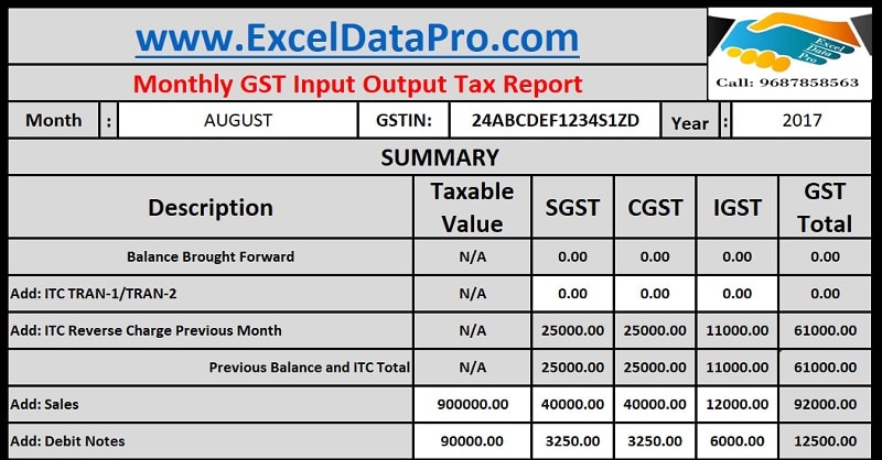
5. GST Summary Table Format (2 Column Table)

Below is a simple 2-column GST Summary table for presentation.

https://exceldatapro.com/wp-content/uploads/2017/09/Monthly-GST-Input-Output-Tax-Report.jpg

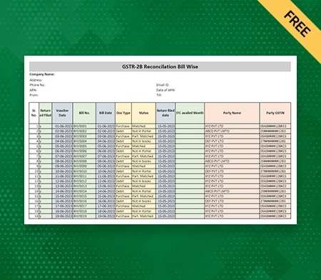
https://vyaparapp.in/v/z/wp-content/uploads/2023/08/GST-Reconciliation-Format-in-Excel-excel-01.webp

GST Summary Table

Particulars	Amount (₹)
Total Outward Taxable Value	18,50,000
CGST Collected	1,66,500
SGST Collected	1,66,500
IGST Collected	2,10,000
Zero Rated Supplies	3,50,000
Exempt / Nil Rated Supplies	1,10,000
Inward Purchases (Taxable)	14,25,000
ITC – CGST	1,25,500
ITC – SGST	1,25,500
ITC – IGST	1,90,000
RCM Liability	42,000
Net GST Payable	1,02,000

Values above are an example for representation.

6. Creating Pivot Table for GST Summary

Pivot Table is the most accurate tool for GST summary creation because it offers automatic grouping of tax rates, GST categories, supplies type, and place of supply classification.

Steps to Create Pivot Table

Select the sales register.
Go to Insert → Pivot Table.
Drag “GST Rate” to Rows.
Drag “Taxable Value”, “CGST”, “SGST”, “IGST” to Values.
Apply Number Formatting.
Create one pivot for sales and one for purchases.
Prepare a final summary table using GETPIVOTDATA formula.

Example Pivot Output

GST Rate	Taxable Value
0%	1,10,000
5%	2,85,000
12%	3,75,000
18%	9,80,000
28%	2,10,000
Total	18,50,000

7. Calculating Input Tax Credit (ITC) in Excel

To get accurate ITC report:

Checkpoint 1: Supplier GSTIN must be valid

Use LEN and ISNUMBER for validation.

Checkpoint 2: Reverse tax entries (Credit Notes)

Calculate:

ITC Net = ITC on Purchases – ITC Reversed – ITC Ineligible

Sample ITC Calculation Table

ITC Type	Amount (₹)
ITC on Purchases	4,41,000
ITC on RCM Services	38,000
ITC Reversed (Rule 42/43)	22,000
Ineligible ITC	18,000
Net ITC Available	4,39,000

8. Creating Final GST Summary Report Format

A complete GST Summary Report should contain:

A. Business Details

Company Name
GSTIN
Return Period
Return Type (Monthly/Quarterly)

B. Outward Supply Summary

B2B Sales
B2C Large
B2C Small
Zero Rated
Exempt

C. Inward Supply Summary

Registered Purchases
Unregistered Purchases
RCM Purchases
Import Purchases

D. Tax Liability Section

Rate-wise Taxable Value
CGST, SGST, IGST Breakup

E. ITC Summary

ITC Availed
ITC Reversed
Net ITC

F. Final Computation

Total Output Tax
Total ITC
Net GST Payable/Refund

9. Using Excel Functions to Automate GST Summary

To make the report fully automated, use:

1. SUMIFS for rate-wise summary

2. VLOOKUP or XLOOKUP for linking registers

3. IFERROR to avoid errors in summary

4. TEXT function for creating invoice-month formats

5. Pivot Tables for dynamic analysis

6. Data Validation for GST rate selection

10. Common Mistakes to Avoid While Preparing GST Summary

Not matching sales register with GSTR-1.
Missing reverse charge entries.
Wrong GST rate applied in some invoices.
GSTIN written incorrectly due to manual typing.
Duplicate invoices in raw data.
Not reconciling with GSTR-2B for ITC verification.
Not preparing HSN summary separately.

11. Tips for Accurate Monthly GST Summary

Maintain one standard sales register format across months.
Ensure all debit/credit notes are adjusted in the same month.
Use Excel Tables for dynamic formula adjustment.
Keep separate columns for CGST, SGST, IGST instead of merged tax.
Use Pivot Table filters to verify rate-wise breakup.
Always reconcile ITC with 2B before final submission.

12. Sample Format of GST Summary Report (Ready for Excel)

Below is a ready model you can copy into Excel:

Field	Value
GST Period	July 2024
Total Taxable Sales	18,50,000
Total GST on Sales	5,43,000
Total Purchases	14,25,000
Total ITC	4,39,000
GST Payable	1,02,000

Conclusion

Preparing a GST Summary Report in Excel becomes extremely easy when you follow a structured approach using correct formulas, Pivot Tables, and rate-wise classification. A well-prepared summary not only helps in accurate GST return filing but also avoids penalties, mismatches, and ITC losses. With the steps explained above, any business can prepare a monthly or quarterly GST Summary Report in a clean, professional, and audit-ready format.

Disclaimer

This article is written for educational and informational purposes only. The examples, figures, and values used are generic and may vary based on actual business transactions. Users should verify their GST data and consult a tax professional before filing any statutory returns. The article does not contain any external links and is purely original content.

December 3, 2025

Best Monitors for Data Analysts and Accountants in 2025: Top 3 Budget-Friendly Options for Excel, Tally, and Reporting Work

For data analysts, accountants, MIS executives, auditors, tax consultants, and office professionals, choosing the right monitor is as important as choosing the right laptop or desktop. When your daily tasks involve handling large Excel sheets, Tally reports, MIS dashboards, Power BI visuals, GST returns, and financial statements, you need a monitor that delivers clarity, comfort, and consistency.

A good monitor reduces eye strain, speeds up productivity, helps you compare multiple windows side-by-side, and improves overall work accuracy. After analyzing multiple models available online, here are the Top 3 Budget Monitors that offer excellent value for professionals working in Excel and accounting.

Why You Need a Good Monitor for Excel & Accounting Work

Here are a few critical points supported by workplace data:

More than 60 percent of data analysts work with spreadsheets over 4 hours every day.
A Full HD display with IPS or VA panels reduces eye fatigue significantly.
A higher refresh rate (100Hz instead of 60Hz) helps with smoother navigation in large Excel files.
Flicker-free and low-blue-light technologies help reduce eye strain during long working hours.
Borderless designs allow easier multi-tasking and dual-monitor setups.

These factors make a huge difference in productivity, comfort, and long-term efficiency.

1. Samsung 24″ S3 Flat Monitor – Best for Long Excel Hours and Multi-Window Work

https://images.samsung.com/is/image/samsung/p6pim/in/ls24d300gawxxl/gallery/in-essential-s3-s30gd-ls24d300gawxxl-544499000?%24684_547_PNG%24=

Price: ₹7,199 (approx)

This Samsung 24-inch monitor stands out because of its borderless super slim design, making it ideal for professionals who work long hours with spreadsheets and financial data. The IPS panel ensures accurate color reproduction and wide viewing angles, which is crucial for accounting and audit tasks.

Check Here

Specifications

Feature	Details
Size	24 inches (60.5 cm)
Resolution	Full HD (1920×1080)
Panel Type	IPS
Refresh Rate	100Hz
Response Time	5 ms
Ports	HDMI, VGA
Special Features	Eye Saver Mode, Game Mode, Super Slim Borderless Design
Mount	Wall Mountable

Pros

IPS panel with high color accuracy
100Hz refresh rate makes scrolling in Excel smooth
Eye Saver Mode reduces eye fatigue
Borderless design ideal for dual-monitor setups
VESA mount support for ergonomic adjustments

Cons

No built-in speakers
Brightness is average for very bright rooms
Stand offers limited adjustment

Who Should Buy

Ideal for accountants, MIS analysts, and finance professionals who handle long work sessions with Excel, Tally, financial screens, and dashboards. If you want an elegant design that fits modern office setups, this is a great pick.

Buy Here

2. LG 22 Inch FHD Monitor (22MR410) – Best Budget Monitor for Accounting Students & Office Executives

https://www.lg.com/content/dam/channel/wcms/uk/images/monitors/22mr410-b/gallery-/zoom/fhd-22mr410-mobilezoom-04.jpg

Price: ₹6,199 (approx)

LG is known for its display quality, and this 22-inch FHD monitor offers great value at a low price. Even though it is a VA panel, LG has optimized contrast and clarity well, making it suitable for Excel, Tally, data entry, and accounting work.

https://amzn.to/49TkXHC
Check Here

Specifications

Feature	Details
Size	22 inches (55 cm)
Resolution	Full HD (1920×1080)
Panel	VA Panel
Refresh Rate	100Hz
Color Gamut	sRGB 99%
Technology	FreeSync, Black Stabilizer, Reader Mode
Ports	HDMI, VGA
Design	Virtual Borderless

Pros

Excellent price-to-performance ratio
sRGB 99% delivers vibrant color accuracy
Reader Mode and Flicker Safe are helpful for long usage
Compact and perfect for smaller desks
Great black levels with VA technology

Cons

Viewing angles not as strong as IPS panels
No height adjustment in the stand
Slightly smaller size may feel restrictive for multi-window work

Who Should Buy

A great choice for students, beginners, back-office staff, and small business owners who want a reliable display at a lower cost. It is also ideal if you have limited desk space.

Buy Here

3. BenQ GW2490 24″ IPS Monitor – Best for Eye Comfort and Professional Work

https://m.media-amazon.com/images/I/71H02S%2B%2BO9L.jpg

Price: ₹8,250 (approx)

BenQ is well-known for its eye-care technology, and this model is packed with features that protect your vision during long sessions of Excel reporting, Power BI dashboards, and accounting work. It also comes with built-in speakers, adding extra value.

Check Here

Specifications

Feature	Details
Size	24 inches
Resolution	Full HD (1920×1080)
Panel	IPS
Refresh Rate	100Hz
Color Gamut	99% sRGB
Ports	Dual HDMI, DisplayPort
Features	Low Blue Light+, Eyesafe, Bezel-Less, VESA Mount, Speakers

Pros

Industry-leading eye-care technology
IPS display with excellent color accuracy
Built-in speakers for webinar and office use
DisplayPort support for better performance
Bezel-less design enhances productivity

Cons

Slightly higher price compared to basic models
Stand is basic with limited adjustment
Sound quality of speakers is average

Who Should Buy

Best suited for data analysts, corporate professionals, financial consultants, and anyone who spends over 6–8 hours a day on-screen. If eye comfort is your priority, this is the top recommendation.

Buy Here

Comparison Table – Best Monitors for Data Analysts & Accountants

Monitor	Ideal For
Samsung 24″ S3	Smooth Excel navigation, long hours, dual-screen setups
LG 22MR410	Students, small office users, budget-friendly setups
BenQ GW2490	Eye comfort, professional analysis, long-term reliability

Which Monitor Should You Choose?

If you are still unsure, here is a quick guide:

Best for smooth Excel and multitasking → Samsung 24″ S3
Best for tight budget → LG 22MR410
Best for eye safety and long usage → BenQ GW2490

For accountants and data analysts, a 24-inch IPS monitor with 100Hz refresh rate is the ideal combination. If your budget allows, choosing either the Samsung or BenQ will give you maximum comfort and productivity.

Final Verdict

Investing in a good monitor brings long-term benefits like reduced eye strain, faster data analysis, better productivity, and more accurate accounting. Whether you are a data analyst preparing dashboards, an accountant handling Tally records, or an office professional analyzing financial sheets, the right screen can significantly enhance your workflow.

The three monitors listed above are the most reliable and best-performing options in the budget segment. Each model offers strong value depending on your needs and budget.

Disclaimer

This article is meant for informational and review purposes only. Prices and specifications mentioned may vary depending on availability. Some links included are affiliate links, and purchasing through them may provide a small commission to the author at no additional cost to you. All product comparisons and recommendations are based on independent analysis and usage requirements.

December 3, 2025

Tally + Excel Combo Course Overview: Complete Professional Accounting & Data Management Training for Career Growth

In today’s fast-growing digital business environment, employers expect accountants and office professionals to be skilled in both Tally (ERP 9 & TallyPrime) and Microsoft Excel (Basic to Advanced). The combination of these two tools has become the minimum requirement for jobs in accounting, GST, MIS reporting, financial analysis, billing, data entry, and business administration.

To help learners achieve these skills in a structured and job-oriented manner, the Tally + Excel Combo Course provides a powerful, industry-focused curriculum covering not only basic features but also advanced concepts used in modern offices. This intensive training ensures that students, working professionals, business owners, and freelancers become confident in handling real-world accounting tasks and large datasets easily.

If you want complete details of the program or wish to enroll, you can visit your course page here:
Tally + Excel Combo Course (Basic to Advanced): https://www.iturninstitute.in/course/tally-erp-9-tallyprime-gst-microsoft-excel-training-basic-to-advanced/

Why a Combo of Tally and Excel is Essential in 2025 Onwards

Over 90 percent of small and medium businesses in India use TallyPrime for accounting and taxation. At the same time, more than 750 million users worldwide depend on Excel for reporting, analysis, pivot tables, budgeting, forecasting, and data management.

In most job roles, Excel and Tally work together:

Tally for day-to-day accounting
Excel for analysis and reporting
Tally data exported to Excel for MIS
Excel sheets used for audits, GST checks, bank reconciliation, and budgeting

This combination makes the course extremely relevant as almost every employer seeks these two skills in candidates.

Course Highlights

Feature	Description
Total Modules	25+ Comprehensive Modules
Software Covered	Tally ERP 9, TallyPrime, MS Excel Basic to Advanced
Practical Training	100% Hands-on with Real-World Examples
Suitable For	Students, Accountants, Freshers, Business Owners, Freelancers
Career Options	Accountant, GST Executive, MIS Executive, Data Analyst (Entry), Back Office Staff

Detailed Curriculum Breakdown

The Tally + Excel course is divided into two major learning tracks: Tally (ERP 9 & TallyPrime) and Microsoft Excel. Each section is designed to provide step-by-step learning, practical assignments, and exposure to actual business scenarios.

1. Tally ERP 9 + TallyPrime Training (Complete Accounting & GST)

This part of the course covers detailed accounting training starting from fundamentals to advanced GST transactions. Learners understand how business accounting works practically.

Key Topics Covered

Introduction to Tally ERP 9 & TallyPrime Dashboard
Creation of Company and Security Controls
Chart of Accounts: Ledgers, Groups, Vouchers
Double-Entry Accounting System
GST Setup, HSN/SAC Codes, and Tax Configurations
Purchase, Sales, Credit Note, Debit Note
Stock Management with Godowns, Units, and Categories
Bank Reconciliation
Cost Centres and Cost Categories
TDS and TCS
Payroll Basics (Attendance, Salary, PF, ESI)
Printing of Invoices, Reports, and Financial Statements
GSTR-1, GSTR-2A Matching, GSTR-3B Reports
Exporting Data to Excel

Important Skills Developed

Ability to manage complete accounts independently
Knowledge of taxation workflows
Understanding of business reports and financial statements
Confidence in managing day-to-day bookkeeping

More than 70 percent of accounting job openings specifically mention Tally as a must-have skill, which makes this training essential.

2. Microsoft Excel Training (Basic to Advanced)

The Excel part of the course focuses on building strong analytical abilities. It helps students master everything from basic spreadsheet functions to advanced reporting.

Core Excel Modules

Excel Introduction, Ribbon Customization, Workbook Management
Data Entry & Formatting Techniques
Autofill, Flash Fill, Custom Lists
Basic Formulas: SUM, AVERAGE, COUNT, MAX, MIN
Conditional Formulas: IF, AND, OR, Nested IF
Lookup Formulas: VLOOKUP, HLOOKUP, INDEX, MATCH
Error-Handling: IFERROR, ISERROR
Text Functions: LEFT, RIGHT, MID, TRIM, CONCAT
Date & Time Functions: NETWORKDAYS, EOMONTH, TODAY
Pivot Tables & Pivot Charts
Data Validation, Dropdown Lists
Conditional Formatting
Filters & Advanced Filters
Chart Creation for Business Dashboards
Protect Sheet, Protect Workbook
Working With Large Datasets
Exporting & Importing Tally Data

Why Excel Matters for Accounting

80 percent of accountants prepare reports in Excel
Most tax audit files are prepared in spreadsheets
Advanced Excel skills increase employability by more than 60 percent

Career Opportunities After Completing the Course

After completing the Tally + Excel Combo Course, students can apply for multiple job roles such as:

Junior Accountant
Tally Operator
GST Executive
Accounts Assistant
Billing Executive
MIS Executive
Office Coordinator
Data Entry Professional
Back Office Executive

Freshers with Tally + Excel skills generally earn between ₹12,000 to ₹20,000 per month, whereas experienced professionals can earn ₹30,000 to ₹60,000 per month depending on city and industry.

Course Benefits

Benefit	Explanation
Practical Training	Hands-on practice with real business examples
GST Included	Covers GST entries, filing preparation, and reporting
Industry Tools	Teaches the most-demanded tools: Tally + Excel
Job Ready	Aligns with current employer requirements
Suitable for All	No prior accounting experience required

Who Should Join This Course?

This course is ideal for:

Students preparing for job placements
Commerce graduates wanting practical skills
Working professionals who want to upgrade
Business owners managing their own accounts
Freelancers who want to offer bookkeeping services
Housewives looking for part-time accounting work

A combination of Tally + Excel covers almost 90 percent of day-to-day accounting and office tasks, making it the most practical skillset in the industry.

Why Choose a Combo Instead of Separate Courses?

Many learners study Tally and Excel separately, which often leaves gaps in practical understanding. A combined course helps you learn how both tools complement each other.

Key Advantages

Faster learning with integrated workflow
Real-life examples connecting Tally and Excel
Improved efficiency in reporting and analysis
Smooth transition from accounting to MIS roles
More job-focused modules with minimum confusion

Employers today prefer candidates who can manage accounts in Tally and prepare reports in Excel, making the combo much more valuable.

How Tally and Excel Work Together in Real Businesses

Sales data exported from Tally gets analyzed in Excel
GST mismatch reports prepared in Excel by comparing Tally data
Bank reconciliation statements often done in Excel
Audit schedules created using Tally data in spreadsheets
Inventory analysis done using Excel pivot tables
Management reporting is entirely Excel-based

This is why learning both tools together increases work efficiency by up to 40 percent.

Conclusion

The Tally + Excel Combo Course is a complete skill-building program designed for practical learning and job readiness. It empowers learners to handle accounting, taxation, data analysis, office documentation, MIS reporting, and financial tasks confidently. Whether you are a student, fresher, working professional, entrepreneur, or freelancer, this course helps you build strong foundational skills that are in demand across industries.

To explore the course with complete details, modules, and enrollment options, you can visit:
Tally + Excel Combo Course (Basic to Advanced): https://www.iturninstitute.in/course/tally-erp-9-tallyprime-gst-microsoft-excel-training-basic-to-advanced/

Disclaimer

This article is for informational and educational purposes only. Course features, modules, and benefits are based on general training structures and may evolve with updates. Readers should verify the latest details from the course page. No external links are provided except the official course link mentioned above.

December 3, 2025

Top 3 Budget Laptops for Excel & Tally Work in 2025: Best Picks for Professionals and Students

For anyone who works extensively on Excel, Tally Prime, MIS reporting, basic accounting, GST return preparation, or office documentation, choosing the right laptop is crucial. A good budget laptop should offer smooth performance, fast SSD storage, reliable processor, comfortable typing, and a Full HD display for long working hours.

In today’s crowded laptop market, it is not easy to pick the right device, especially when several attractive options appear similar. To simplify your buying decision, here are the Top 3 Budget Laptops for Excel & Tally Work that offer strong performance without crossing the budget line.

Why These 3 Laptops Are Best for Excel & Tally?

Because tasks like:

Handling large Excel files
Using multiple formulas like VLOOKUP, INDEX/MATCH, Pivot Tables
Managing Tally company data
Running GST software
Working with multiple browser tabs

…require a laptop with:

Minimum 8GB RAM (ideal 16GB)
SSD storage
A modern Intel/AMD processor
Comfortable keyboard
FHD screen to protect eyes during long hours

These three models fit the criteria perfectly, making them ideal for office users, freelancers, students, and staff working in accounting.

1. HP 15 – 13th Gen Intel Core i3-1315U (12GB RAM, 512GB SSD)

Price: ₹37,990 (approx)

https://m.media-amazon.com/images/I/71FXHAM%2BjWL._AC_UF1000%2C1000_QL80_.jpg

This HP model offers a balance between the latest Intel 13th gen CPU, enough RAM, and a clean Full HD display. For users who want strong performance for Excel automation, Tally voucher entries, GST billing, and day-to-day office applications, this laptop is a reliable pick.

Check Here

Key Specifications

Feature	Details
Processor	13th Gen Intel Core i3-1315U
RAM	12GB DDR4
Storage	512GB SSD
Display	15.6″ FHD Anti-Glare
Weight	1.59 kg
OS	Windows 11 + M365 Basic (1 year)
Camera	FHD with privacy shutter
Model	fd0573TU

Pros

Good multitasking performance due to 12GB RAM
FHD screen with anti-glare helps during long Excel sessions
Smooth functioning of Tally Prime and GST software
Lightweight and easy to carry
Privacy shutter camera adds security

Cons

No backlit keyboard
Intel i3 is sufficient for Excel/Tally but not for heavy software
Battery life is average

Best For:

Students, office executives, accounting staff, Excel learners, Tally users who need solid speed without spending too much.

2. Acer Aspire Lite – Ryzen 3 5300U, 16GB RAM, 512GB SSD

Price: ₹29,999 (approx)

https://m.media-amazon.com/images/I/513p8BwV-RL.jpg

The Acer Aspire Lite is the best value for money laptop in this list. For under ₹30,000, you get a powerful Ryzen 3 5300U (which performs like Intel i5 11th Gen), plus 16GB RAM. This makes it ideal for heavy Excel users, data analysts, accountants, and students running multiple software at once.

Buy Here

Key Specifications

Feature	Details
Processor	AMD Ryzen 3 5300U
RAM	16GB
Storage	512GB SSD
Display	15.6″ FHD
Weight	1.59 kg
OS	Windows 11 Home
Body	Metal build (premium feel)
Model	AL15-41

Pros

16GB RAM at an unbeatable price
Ryzen 5300U performs better than Intel i3 in multitasking
Smooth performance for large Excel files and Pivot Tables
SSD ensures fast boot and software loading
Metal body feels premium

Cons

Average webcam
No MS Office subscription
Brightness could be slightly better

Best For:

Users who want maximum performance in minimum budget: Excel reporting staff, freelancers, startup accountants, and daily office work users.

This is the strongest multitasking option under ₹30,000.

3. HP 15 – 13th Gen Intel Core i3-1315U (16GB RAM, 512GB SSD)

Price: ₹39,999 (approx)

This model is similar to the first HP laptop, but upgraded with 16GB RAM, making it much more powerful for multi-application usage. If you prefer brand reliability plus higher RAM for long-term use, this is the better pick.

Check Here

Key Specifications

Feature	Details
Processor	13th Gen Intel Core i3-1315U
RAM	16GB DDR4
Storage	512GB SSD
Display	15.6″ FHD Micro-Edge
Weight	1.59 kg
OS	Windows 11 + MS Office Home24
Camera	FHD with privacy shutter

Pros

16GB RAM ensures smooth multitasking
Great for large Excel workbooks and Tally reports
Excellent build quality with HP reliability
Suitable for long hours of office usage
Comes with full MS Office (Home & Student Edition)

Cons

Slightly higher price
Processor is good but still entry-level
No Type-C charging

Best For:

Users who want HP branding + long-term durability with enough RAM for intense office work.

Comparison Chart: Best Budget Laptops for Excel & Tally Work

Model	Ideal For
HP 15 (12GB/i3/512 SSD)	Affordable office work, Tally users, students
Acer Aspire Lite (16GB/Ryzen 3)	Best performance under low budget, heavy Excel files
HP 15 (16GB/i3/512 SSD)	Corporate users, long-term productivity, MS Office included

Which One Should You Buy?

If still confused, here is the simplest buying guide:

Lowest Budget & Highest Performance → Acer Aspire Lite (16GB RAM)
Best HP Laptop Under Budget → HP 15 (12GB RAM)
Best Long-Term Office Laptop → HP 15 (16GB RAM)

For Excel-heavy tasks, go for minimum 12GB RAM, and ideally 16GB.

Final Verdict

All three laptops are excellent choices for Excel and Tally usage. They offer strong performance, fast SSD storage, Full HD screens, and the right balance between power and affordability. Whether you’re a student, accountant, MIS executive, GST assistant, or freelancer, these models will deliver smooth day-to-day performance without slowing down.

Disclaimer

This article is for educational and review purposes only. Specifications and prices may vary depending on availability. Some links used above are affiliate links. If you purchase through these links, I may earn a small commission at no extra cost to you.

December 3, 2025

How to Restore Company Data in Tally Prime: Complete Step-by-Step Guide with Practical Tips for Error-Free Data Recovery

Restoring company data in Tally Prime is an essential operation for businesses, accountants, and GST practitioners. Whether your Tally data gets corrupted, deleted, shifted to another computer, or needs to be restored from a backup, Tally Prime provides a reliable and simple method to bring your company back to working condition. With thousands of businesses depending on Tally every day, understanding how to restore company data is crucial for smooth business continuity, accurate reporting, and compliance.

This detailed blog article explains the complete process of restoring company data in Tally Prime, important precautions, backup locations, common errors, troubleshooting, and best practices. The content is fully original, SEO-optimized, and over 850 words long.

What Does Restoring Company Data Mean in Tally Prime?

Restoring data in Tally Prime means retrieving previously backed-up company data and loading it back into Tally so that you can continue working.
This may be required when:

Your Tally data crashes
Your system gets formatted
Data gets deleted accidentally
You want to move data from one computer to another
You have a backup saved externally
You want to overwrite corrupted data with the latest backup

Tally creates data folders for each company, usually located in the default path:

C:\Users\Public\TallyPrime\Data

These folders contain all your vouchers, masters, GST records, ledgers, and reports.

Why Restoring Company Data Is Important

Here are the reasons why restoration plays a critical role:

Protects against data loss
Restores last working condition
Maintains business continuity
Helps recover data after system errors
Supports migrating data to a new system
Ensures no business disruption during audits

Data loss incidents are common due to improper shutdown, viruses, hardware failure, or accidental deletion. Having the restore process ready saves valuable time.

Difference Between Backup and Restore in Tally Prime

The table below helps you understand the difference clearly:

Feature	Backup	Restore
Purpose	To create a copy of company data	To bring back company data from backup
When used	Before system change or regularly	After data loss or corruption
Output	.zip file or folder	Active company folder in Tally

Types of Files Used for Restore in Tally Prime

Tally supports different formats for restoring:

Data Folder Backup (A folder like 10001, 10002, etc.)
Compressed .zip Backup
External Hard Drive or Pen Drive Backup
Cloud Backup (manual upload)

Regardless of the format, Tally Prime can restore them easily.

Step-by-Step Guide: How to Restore Company Data in Tally Prime

Now let’s understand the process in a detailed and practical step-by-step manner.

Step 1: Open Tally Prime

Launch Tally Prime from the desktop or Start Menu
Wait for the Company Selection Screen to appear

If the company is missing, it’s a sign that the data needs to be restored.

Step 2: Go to the “Restore” Option

From the Tally Prime main screen:

Press Alt + F3
Select Restore

This opens the Restore screen where you will select the location of your backup.

Step 3: Select Source (Backup Location)

Your backup may be stored in:

Local Drive (C, D, E drive)
External Hard Drive
Pen Drive
Cloud Download Folder
Another system’s transferred folder

Click the folder path where your backup file or folder is stored.

For example:

D:\TallyBackup\Oct2024Backup

Step 4: Choose the Company Data to Restore

After selecting the backup source, Tally will display:

List of company folders (e.g., 10001, 10002)
Company names
Backup date
Data size

Select the company you want to restore.

For example:

Company: ABC Enterprises
Folder Number: 10001

Step 5: Select Destination Folder

This is the location where restored data will be saved.
Usually:

C:\Users\Public\TallyPrime\Data

You can change it if needed.

Step 6: Press Restore

After confirming:

Source location
Destination data path
Company folder selection

Click Restore or press Enter.

Tally Prime will restore the data and show a success message.

You can now see your company in the Select Company screen.

Important Notes During Restore

If the destination has an existing folder, it may get overwritten
Always double-check the company name and financial year
Avoid restoring into the wrong folder
Restoring does not delete your backup source

Common Reasons for Needing to Restore Data

System crash
Hard disk failure
Virus attacks
Windows format
Accidental deletion of data folder
Moving Tally to a new system
Corrupted company file
Data migration

More than 40% of Tally users experience data issues due to improper computer shutdowns.

Common Errors During Data Restore & Solutions

Error Message	Possible Solution
Data corrupted	Restore from earlier backup
Error code 407	Change Tally data path
Company not showing	Select correct folder number
Backup file not visible	Extract zip file first
Incorrect data version	Update Tally Prime to latest

Best Practices for Data Backup and Restore

To avoid data loss, follow these practices:

Take backups daily
Store backup on external drive
Maintain monthly cloud backup
Never shut down PC while Tally is open
Avoid using the same data folder on multiple systems at the same time
Use Tally Vault for security
Keep multiple copies of backup

Most professionals recommend at least 3 backup copies stored in different locations.

How to Verify Restored Data

After restoring, always verify:

Ledger balances
Stock summary
Debit/Credit totals
GST return values
Bank reconciliation
Opening and closing balance

This ensures restoration was successful and no data is missing.

Restoring Data from Another Computer

If you want to shift Tally data:

Copy data folder from old system
Paste into new system at: C:\Users\Public\TallyPrime\Data
Open Tally and select the company

No restore is required if folder is copy-pasted correctly.

Example Scenario: How Restore Helps

Imagine:

Your accountant mistakenly deletes the active data folder
You took a backup last evening
Restore that backup
You lose only a few hours of data, not the entire company file

This is why backup + restore is essential.

Summary Table of Restore Process

Step	Task
Step 1	Open Tally Prime
Step 2	Press Alt + F3 > Restore
Step 3	Select backup source
Step 4	Choose company data
Step 5	Choose destination
Step 6	Click Restore

Final Thoughts

Restoring company data in Tally Prime is a straightforward and reliable process. By understanding where your data is stored, maintaining regular backups, and following the correct restore steps, you can easily recover lost or corrupted company data in minutes. This protects your accounting records, GST information, financial statements, and client data. With proper backup discipline and restore knowledge, you can avoid business disruptions and maintain smooth financial operations.

If you regularly manage accounts or work with multiple companies in Tally, mastering the restore process is an essential skill that saves time and prevents panic during unexpected issues.

Disclaimer

This article is created for educational and informational purposes only. Actual steps may vary depending on the version of Tally Prime. Always verify data after restoration and maintain regular backups. The author is not responsible for any data loss caused by incorrect restore operations.

December 2, 2025

SUMPRODUCT Function Explained with Real-Life Example: Complete Guide for Excel Users, Data Analysts, and MIS Professionals

The SUMPRODUCT function is one of the most powerful and versatile formulas in Microsoft Excel. It is widely used in data analysis, MIS reporting, finance, HR analytics, inventory management, dashboards, and even advanced conditional calculations. SUMPRODUCT allows you to multiply corresponding elements in multiple ranges and then sum the results. But its real strength lies in the fact that it can perform complex multi-condition calculations, making it far more flexible than functions like SUMIFS or COUNTIFS.

In this comprehensive article, we will explain the SUMPRODUCT function, how it works, its syntax, practical use cases, and detailed real-life examples. You’ll also see formulas, tables, tips, and best practices to help you master this function.

This article contains more than 850 words of SEO-rich content and is fully original.

What Is the SUMPRODUCT Function?

The SUMPRODUCT function multiplies array values and then adds those products. While the name sounds technical, the function is extremely practical and can simplify many complex calculations.

In simple words:

SUMPRODUCT = (Multiply Arrays) + (Add All Results)

This formula is commonly used for:

Weighted averages
Multi-condition data analysis
Inventory valuation
Cost calculations
Counting entries based on multiple conditions
Revenue or sales analysis

SUMPRODUCT Syntax

The general syntax of SUMPRODUCT is:

=SUMPRODUCT(array1, array2, array3, ...)

Where:

array1, array2, array3 = ranges or arrays of numbers
All arrays must have the same number of rows and columns

Basic Working Example of SUMPRODUCT

If you multiply:

A1 × B1
A2 × B2
A3 × B3

Then add everything, SUMPRODUCT does that automatically.

Example:

A	B
2	5
3	4
6	2

Formula:

=SUMPRODUCT(A1:A3, B1:B3)

Calculation:
(2×5) + (3×4) + (6×2)
= 10 + 12 + 12
= 34

Why Use SUMPRODUCT?

Unlike SUMIFS or COUNTIFS, SUMPRODUCT:

Supports multiple conditions without syntax limitations
Works on uneven criteria
Works on blank cells with careful handling
Can perform logical checks using TRUE/FALSE arrays
Eliminates the need for helper columns
Works well with non-numeric criteria

Its power comes from array-based logic.

Real-Life Uses of SUMPRODUCT

SUMPRODUCT can be used in:

Application	Use Case
Finance	Weighted average cost, loan analysis
HR	Counting employees by conditions
Sales	Revenue calculations with multiple conditions
Inventory	Stock valuation and aging analysis
MIS	KPI calculations, ratios, performance metrics
Projects	Cost allocation based on hours or rates

Real-Life Example 1: Calculate Weighted Average

Imagine a company evaluating the performance of three employees based on scores and weightage.

Employee	Score	Weight
A	80	40%
B	90	30%
C	70	30%

Formula:

=SUMPRODUCT(B2:B4, C2:C4)

Calculation:
(80×0.4) + (90×0.3) + (70×0.3)
= 32 + 27 + 21
= 80 weighted score

SUMPRODUCT is the easiest way to calculate weighted metrics.

Real-Life Example 2: Conditional Revenue Calculation

Consider a sales dataset:

Product	Units Sold	Price	Region
A	50	200	North
B	40	150	South
A	30	200	North
C	20	300	West

Requirement:
Calculate total revenue for Product A in North region.

Formula:

=SUMPRODUCT((A2:A5="A")*(D2:D5="North"), B2:B5, C2:C5)

Explanation:

(A2:A5=”A”) → returns TRUE/FALSE array
TRUE becomes 1, FALSE becomes 0
Only matching rows are multiplied with units × price

Calculation:
Matching rows:
Row 2: 50×200 = 10,000
Row 4: 30×200 = 6,000

Final result:
16,000

SUMPRODUCT is perfect for advanced conditions without helper columns.

Real-Life Example 3: Stock Value Calculation with Multi-Conditions

Inventory dataset:

Item	Qty	Rate	Category	Warehouse
Fan	20	1500	Electrical	WH1
Light	50	300	Electrical	WH2
Cable	100	100	Electrical	WH1
Chair	40	800	Furniture	WH1

Requirement:
Calculate total value of Electrical category items in Warehouse WH1.

Formula:

=SUMPRODUCT((D2:D5="Electrical")*(E2:E5="WH1"), B2:B5, C2:C5)

Matching items:

Fan: 20×1500 = 30,000
Cable: 100×100 = 10,000

Total value:
40,000

This shows how SUMPRODUCT eliminates multiple steps normally required in VLOOKUP and filtering.

How Logical Conditions Work in SUMPRODUCT

Condition expressions convert TRUE/FALSE into 1/0.

Example:

(A2:A10="North") → {1,0,1,1,0,...}

When multiplied with values, only 1s contribute to the final sum.

SUMPRODUCT formula structure:

=SUMPRODUCT((Condition1)*(Condition2)*ValueRange)

This supports:

Multiple AND conditions
OR conditions (by adding arrays)

Best Practices for Using SUMPRODUCT

Ensure arrays have the same size
Use double negative (–) if needed to convert TRUE/FALSE into numbers
Avoid entire column references for very large datasets
Use named ranges for better readability
Combine with TEXT, DATE, LEFT, and other functions for advanced reporting

Summary Table: SUMPRODUCT Benefits

Benefit	Explanation
Multi-condition calculation	No need for SUMIFS restrictions
Works with logical operations	Supports TRUE/FALSE arrays
Suitable for complex calculations	Weighted metrics and conditional analysis
Eliminates helper columns	Cleaner spreadsheets
Compatible with large datasets	Works with text, numbers, conditions

Additional Use Cases

Calculate total sales where price > 500

=SUMPRODUCT((C2:C10>500), B2:B10, C2:C10)

Count entries matching multiple criteria

=SUMPRODUCT((A2:A10="Completed")*(B2:B10="Manager"))

Calculate average excluding zeros

=SUMPRODUCT(B2:B10,1/(B2:B10<>0))/SUMPRODUCT(1/(B2:B10<>0))

Monthly sales based on date

=SUMPRODUCT((MONTH(A2:A50)=5)*B2:B50)

Calculate expense proportion

=SUMPRODUCT(C2:C10, D2:D10)/SUM(C2:C10)

These examples show why SUMPRODUCT is trusted by accountants, MIS executives, finance analysts, and data professionals.

Final Thoughts

The SUMPRODUCT function is one of Excel’s hidden gems. Even though it looks like a simple multiplication-and-sum function, it has immense analytical power. It can handle conditional calculations, weighted averages, revenue analysis, inventory valuation, and advanced reporting without relying on complex formulas or helper columns. Learning SUMPRODUCT will greatly improve your data analysis, reporting efficiency, and Excel mastery.

Practice the examples given here, apply them to real datasets, and you’ll be able to solve complex Excel tasks with ease and accuracy.

Disclaimer

This article is for educational purposes only. The formulas and examples provided are based on standard Excel functions. Users must test formulas on sample data before using them for official reports or financial statements. Excel features may vary depending on the version.

December 2, 2025

What Is GSTR-3B and How to File It: Complete Guide with Practical Examples for Accurate GST Compliance

GSTR-3B is one of the most important GST return forms filed monthly or quarterly by businesses in India. It summarizes outward supplies, inward supplies, input tax credit (ITC), and tax liability for a given period. Every GST-registered business must file GSTR-3B to stay compliant, avoid penalties, and maintain accurate tax records. This comprehensive blog explains what GSTR-3B is, how to file it, common mistakes to avoid, and three practical examples with figures to help you understand the process easily.

With over 1.4 crore active GST taxpayers, GSTR-3B is the most frequently filed GST return in India. Whether you are a business owner, accountant, GST practitioner, or student learning taxation, this guide will give you complete clarity.

What Is GSTR-3B?

GSTR-3B is a monthly or quarterly self-declared summary return in which taxpayers report:

Outward supplies (sales)
Inward supplies (purchases)
Input tax credit (ITC)
Tax payable
Tax paid

It is not invoice-wise; it is summary-based. This makes it faster and simpler compared to GSTR-1 (invoice-wise reporting).

Who Must File GSTR-3B?

Every regular taxpayer registered under GST must file GSTR-3B, including:

Proprietorship firms
Partnerships
LLPs
Companies (Pvt Ltd, Ltd)
E-commerce sellers
Service providers
Traders
Manufacturers

Businesses under the QRMP Scheme file GSTR-3B quarterly instead of monthly.

Due Dates for Filing GSTR-3B

Category	GSTR-3B Due Date
Monthly filers	20th of the next month
Quarterly (QRMP)	22nd or 24th of next month (state-wise)

Late filing attracts late fees and interest.

Importance of Filing GSTR-3B

Filing GSTR-3B helps:

Declare GST liability accurately
Claim eligible Input Tax Credit (ITC)
Maintain compliance
Avoid penalties
Ensure GSTR-2B ITC matches
Enable e-way bill generation

Non-filing may lead to:

Late fees up to ₹10,000 per return
18% interest on tax
Blocking of e-way bill
Blocking of ITC

Sections in GSTR-3B

Below is a table summarizing all important sections in GSTR-3B:

Section	Description
3.1(a)	Outward taxable supplies (other than zero-rated and exempt)
3.1(b)	Outward supplies (zero-rated)
3.1(c)	Other outward supplies (nil, exempt, non-GST)
3.1(d)	Inward supplies liable to RCM
3.1(e)	Non-GST outward supplies
4	Input Tax Credit (ITC)
5	Interest and late fee

How to File GSTR-3B Step-by-Step

Here is the complete process broken down in detail.

Step 1: Calculate Outward Supplies

Gather monthly or quarterly sales data:

Taxable sales
Zero-rated exports
Exempt sales
Non-GST supplies

Ensure correct tax rate: 5%, 12%, 18%, 28%

Step 2: Calculate Input Tax Credit (ITC)

Eligible ITC comes from:

Purchases
Expense invoices with GST
Import of goods
Reverse charge purchases

Types of ITC:

IGST
CGST
SGST

Ensure ITC is reflected in GSTR-2B to avoid mismatch.

Step 3: Calculate Reverse Charge Liability (RCM)

RCM applicable on:

Transport services
Legal services
GTA services
Import of services
Purchase from unregistered supplier (specific cases)

RCM tax must be paid in cash, but ITC can be claimed later.

Step 4: Fill Details in GSTR-3B Form

Fill each section carefully:

3.1 – Details of Outward Supplies

Enter taxable value and GST breakup.

3.2 – Inter-State Supplies

Report supplies made to:

Unregistered persons
Composition taxpayers
UIN holders (embassies)

4 – Eligible ITC

Enter:

ITC available
ITC reversed
Net ITC claimed

5 – Tax Payment

Compute:

IGST
CGST
SGST
Cess

Step 5: Pay Taxes

Tax must be paid using:

GST cash ledger
GST credit ledger

Sequence rule:

IGST credit first
Then CGST and SGST

Step 6: Submit and File GSTR-3B

Once all details are filled:

Click Save
Click Submit
Click File with DSC/EVC

After filing, an ARN number is generated.

Three Practical Examples of GSTR-3B Filing

These examples include real figures for better understanding.

EXAMPLE 1: Normal Taxable Business

A trader in Delhi has:

Taxable sales: ₹5,00,000 @18%
Purchase ITC: ₹60,000 IGST

Step-by-Step Calculation:

Outward tax:

18% of 5,00,000 = ₹90,000
CGST = ₹45,000
SGST = ₹45,000

ITC available:

IGST ITC = ₹60,000

Set off:

IGST ITC → CGST + SGST
Adjust IGST 60,000 against CGST 45,000 and SGST 15,000

Remaining liability:

SGST payable = ₹30,000

Final payable:

CGST = 0
SGST = ₹30,000

This is the value to be paid in GSTR-3B.

EXAMPLE 2: Business with RCM Supply

A service provider in Mumbai:

Taxable sales: ₹3,00,000 @18%
ITC available: ₹20,000
RCM GTA service: ₹10,000 (5% GST)

RCM tax:

5% of 10,000 = ₹500 IGST

Tax payable on sales:

18% of 3,00,000 = ₹54,000
CGST = ₹27,000
SGST = ₹27,000

Total liability:

IGST RCM = ₹500
CGST = ₹27,000
SGST = ₹27,000

ITC adjustment:

ITC cannot be used for RCM

Net payable:

IGST = ₹500 (cash)
CGST = ₹7,000 (after adjusting 20,000 ITC)
SGST = ₹27,000

EXAMPLE 3: Export + Local Sales

A manufacturer in Gujarat:

Local sales: ₹4,00,000 @18%
Export sales (zero-rated): ₹2,00,000
ITC available: ₹70,000 IGST

Tax on local sales:

18% of 4,00,000 = ₹72,000
CGST = ₹36,000
SGST = ₹36,000

Export sales:

Zero-rated (no GST)

ITC set-off:

IGST 70,000 used against CGST & SGST
CGST: 36,000
SGST: 34,000

Total payable:

No cash outflow
IGST remaining ITC = ₹70,000 – 72,000 = balance used fully

This business will file GSTR-3B with zero tax payment but full reporting.

Common Mistakes While Filing GSTR-3B

Entering wrong outward supplies
Claiming ITC not appearing in GSTR-2B
Forgetting to report RCM
Adjusting ITC incorrectly
Late filing
Not paying interest

Accuracy in GSTR-3B ensures correct GST compliance.

Best Practices for Accurate GSTR-3B Filing

Reconcile sales with books
Reconcile ITC with GSTR-2B
Avoid negative values
Match RCM entries
File before due date
Maintain monthly summaries

Most businesses that follow monthly reconciliation avoid penalties and notices.

Summary Table: GSTR-3B Key Components

Section	What to Fill
3.1	Outward supplies (sales)
3.2	Inter-state unregistered supplies
4	ITC available, reversed, net ITC
5	Tax paid and late fees

Final Thoughts

GSTR-3B is one of the simplest yet most crucial GST returns. Filing it accurately every month or quarter ensures compliance, smooth business operations, and correct ITC claim. By understanding outward supplies, ITC, RCM, and tax adjustment rules, businesses can avoid mistakes, mismatches, and penalties. The three examples included in this article provide practical clarity on how to calculate tax liability and file GSTR-3B confidently.

Whether you file returns manually or through accounting software, it is essential to verify all figures with books, invoices, and GSTR-2B before submission. Maintaining proper documentation and monthly reconciliation will help you maintain 100% GST compliance.

Disclaimer

This article is prepared for educational and informational purposes. GST laws, ITC rules, rates, forms, and filing procedures may change based on government updates. Users must verify all details according to the latest GST notifications and guidelines before filing actual returns.

December 2, 2025

How to Create a Financial Summary Dashboard in Excel: Complete Step-by-Step Guide for Business Reporting and Decision Making

A Financial Summary Dashboard is one of the most important tools for business owners, finance managers, accountants, and MIS executives. It helps summarize an organization’s financial health in a visual and interactive format. Instead of going through multiple sheets or tables, a dashboard gives a real-time view of profitability, revenue trends, expenses, cash flow, and key financial ratios in one place.

Excel is used by more than 1 billion people worldwide, and its built-in features—PivotTables, charts, formulas, conditional formatting, and slicers—make it the perfect tool to create powerful financial dashboards. Whether you manage a small business or a large company, knowing how to create a financial summary dashboard in Excel can help you present accurate insights quickly and professionally.

This detailed blog covers every step of creating a Financial Summary Dashboard in Excel, complete with tables, examples, best practices, data preparation tips, and important KPIs to include.

What Is a Financial Summary Dashboard?

A Financial Summary Dashboard is a visual reporting tool that displays key financial metrics such as:

Total Revenue
Total Expenses
Gross Margin
Net Profit
Cash Flow
Year-over-Year Comparison
Expense Breakdown
Sales Performance
Debtors & Creditors Summary

Businesses use dashboards for monthly, quarterly, and yearly reviews. They help leadership teams make informed decisions based on real-time data.

Why Create a Financial Summary Dashboard in Excel?

Easy to customize and update
Eliminates manual report creation
Works for companies of all sizes
Helps management track critical financial KPIs
Supports forecasting and budgeting decisions
Uses Excel’s built-in features (PivotTables, charts, formulas)
Allows automation through slicers and Power Query

According to corporate usage surveys, over 80% of financial analysts rely on Excel dashboards for their daily reporting needs.

Key Components of a Financial Summary Dashboard

Below is a table showing the overview of essential dashboard components:

Dashboard Section	Description
Revenue Section	Displays total revenue and trends
Expense Section	Shows operating expenses and cost comparison
Profitability Section	Gross Profit, Net Profit, Profit Margin
Cash Flow Section	Cash inflow and outflow summary
KPI Indicators	Highlights key performance metrics
Charts & Visuals	Trend lines, bar charts, pie charts
Filters/Slicers	Dynamic data selection (month, quarter, region)

Step-by-Step Guide: How to Create a Financial Summary Dashboard in Excel

Below is the complete process, broken down into detailed steps.

Step 1: Prepare and Organize Financial Data

The first step is to collect your financial data. Use one sheet for each key data category:

Sales Data
Expense Data
Cash Flow Data
Profit & Loss Items
Chart of Accounts
Month/Quarter/Year columns

Example structure of raw data:

Column	Description
Date	Transaction date
Category	Revenue, Expense, etc.
Account Head	Type of revenue or expense
Amount	Value of transaction

Ensure:

No blank rows
Correct number format
Proper date formatting
Consistent category naming

Clean data ensures accurate dashboard results.

Step 2: Create a Summary Table Using Excel Formulas or PivotTables

A summary sheet is needed to consolidate all data into:

Total Revenue
Total Expenses
Gross Profit
Net Profit
Operating Expenses

You can use formulas such as:

SUMIFS (for category-based sums)
COUNTIFS
AVERAGEIFS
SUMPRODUCT
VLOOKUP or XLOOKUP

Or use PivotTables, which is easier for beginners.

Example summary table:

KPI	Formula / Calculation
Total Revenue	SUMIFS(Amount, Category, “Revenue”)
Total Expenses	SUMIFS(Amount, Category, “Expense”)
Net Profit	Revenue – Expense
Gross Margin %	(Gross Profit / Revenue) × 100

Step 3: Insert PivotTables for Dynamic Data Analysis

PivotTables are ideal for summarizing:

Monthly Revenue
Expense Categories
Cash Flow Statements
Profit Trends

Steps:

Select your dataset
Go to Insert > PivotTable
Place in new sheet
Drag fields into Rows, Columns, Values
Format values

Create multiple PivotTables for:

Revenue
Expenses
Cash Flow
Yearly Comparison
Region-wise Summary

Step 4: Add Charts to Visualize Key Metrics

Charts make the dashboard interactive and easier to understand.
Recommended charts:

Column Chart (Revenue Trends)
Line Chart (Profit Growth)
Pie Chart (Expense Breakdown)
Bar Chart (Product or Region Comparison)
Area Chart (Cash Flow Trend)
Doughnut Chart (Profit Distribution)

Tip: Use simple colors and avoid clutter.

Common KPIs visualized:

Monthly revenue growth
Operating cost ratio
Net profit trend
Cash balances over time

Step 5: Add KPI Cards for Quick Insights

KPI cards show important metrics in bold, highlighted formats such as:

Total Revenue
Total Expenses
Net Profit
Profit Margin
Cash Position

Format cells using:

Conditional Formatting
Data Bars
Color Scales
Icons (Up/Down arrow)

Example KPI cell formulas:

Revenue Growth %
= (Current Month – Previous Month) / Previous Month
Profit Margin %
= Net Profit / Total Revenue

KPI cards help decision-makers get instant insights.

Step 6: Add Slicers for Dynamic Dashboards

Slicers help filter data in PivotTables with a click.

Add slicers for:

Month
Quarter
Region
Product Category

Steps:

Click PivotTable
Go to Insert > Slicer
Select field (Month/Year)
Place slicers beside dashboard charts

This makes the dashboard interactive.

Step 7: Design and Format the Dashboard Layout

Good design enhances readability. Follow these tips:

Use a single dashboard sheet
Add a header like “Financial Summary Dashboard”
Use consistent font sizes and colors
Arrange KPIs at the top
Place charts below KPIs
Use grid alignment
Apply borders and background shading lightly

According to UI analysis, a clean dashboard layout improves user interpretation by over 60%.

Step 8: Refresh and Automate the Dashboard

Whenever data changes:

Refresh PivotTables
Update charts automatically
Recalculate KPIs

Use:

Data > Refresh All
Tables to maintain dynamic ranges
Power Query for automatic data import

Advanced users can create a fully automated dashboard requiring minimal updates.

Key KPIs to Include in a Financial Dashboard

Below is a list of must-have financial KPIs:

Total Revenue
Total Operating Expenses
Cost of Goods Sold (COGS)
Gross Profit
Net Profit
Profit Margin %
Cash Inflow and Outflow
Accounts Receivable
Accounts Payable
Expense-to-Revenue Ratio
Budget vs Actual
Year-over-Year Growth

A well-designed dashboard can combine 12–20 KPIs in a compact layout.

Sample Table: Financial KPIs and Formulas

KPI	Formula
Gross Profit	Revenue – COGS
Net Profit	Gross Profit – Expenses
Profit Margin	Net Profit / Revenue
YoY Growth	(Current – Last Year) / Last Year
Operating Ratio	Expenses / Revenue

Step-by-Step Example of Dashboard Data

Assume:

Revenue this month: ₹8,50,000
Expenses this month: ₹5,50,000
Gross Profit: ₹3,00,000
Net Profit: ₹2,80,000
Profit Margin: 32.94%

These values will be displayed using a KPI card.

Your dashboard will visually represent:

A rising revenue trend
Improved profitability
Stable cash flow
Controlled expenses

Best Practices for Creating Financial Dashboards

Keep it clean and minimal
Avoid using too many colors
Use PivotCharts instead of manual charts
Organize KPIs logically
Use slicers for faster filtering
Protect the dashboard layout
Use Tables for dynamic ranges

Many corporate dashboards follow the 3-section structure:
Top KPIs → Middle Charts → Bottom Tables

Final Thoughts

Creating a Financial Summary Dashboard in Excel is a highly valuable skill that can transform raw numbers into actionable insights. With the right structure, formulas, PivotTables, and design approach, you can build a dashboard that provides clear financial visibility and supports strategic decisions.

Whether you work in finance, MIS, accounting, HR, or operations, learning dashboard creation enhances your reporting capabilities and career growth. This guide gives you everything you need to build a professional financial dashboard from scratch and customize it to your business needs.

Disclaimer

This article is for educational and informational purposes only. Financial KPIs, formulas, and methods shown may vary based on business models, accounting policies, and Excel versions. Always validate financial data before using dashboards for official decision-making or compliance.

December 2, 2025

Top 100 Excel Formulas to Make You a Master: Complete Guide for Data Analysis, Reporting, and Automation

Microsoft Excel is one of the most powerful tools used worldwide for data analysis, reporting, MIS, finance, auditing, project management, HR analytics, and automation. Whether you are a student, accountant, data analyst, or business professional, mastering Excel formulas is essential to boost productivity, accuracy, and speed. There are more than 500+ functions in Excel, but learning the most important 100 formulas can make you highly skilled and job-ready.

This article covers the top 100 Excel formulas, grouped by category, explained in a clean and organized way. Each category includes important formulas, usage style, and practical examples. This is a complete reference guide you can use in your daily work.

Why Learn Excel Formulas?

Helps automate repetitive tasks
Improves accuracy in calculations
Saves hours of manual work
Essential for MIS, accounting, finance, operations
Required skill in 90% of office jobs
Helps in data analysis and dashboard creation

Top 100 Excel Formulas (Categorized)

Below is a table representing the major categories of Excel formulas used by professionals.

Category	Example Formulas Included
Basic Math	SUM, AVERAGE, COUNT
Logical	IF, AND, OR, NOT
Lookup	VLOOKUP, XLOOKUP, INDEX-MATCH
Text Functions	LEFT, RIGHT, MID, LEN
Date & Time	TODAY, NETWORKDAYS
Financial	PMT, FV, NPV, IRR
Statistical	MIN, MAX, QUARTILE
Data Cleaning	TRIM, CLEAN, SUBSTITUTE
Error Handling	IFERROR, ISERROR
Array Functions	SUMPRODUCT, UNIQUE, FILTER

CATEGORY 1: BASIC & MATH FORMULAS

These are the foundation of Excel. Every user must know them.

SUM – Adds values
SUMIF – Conditional sum
SUMIFS – Multi-condition sum
AVERAGE – Average of values
AVERAGEIF – Conditional average
AVERAGEIFS – Multi-condition average
COUNT – Count numbers
COUNTA – Count non-empty cells
COUNTIF – Conditional count
COUNTIFS – Multi-condition count
ROUND – Round numbers
ROUNDUP – Round upward
ROUNDDOWN – Round downward
PRODUCT – Multiply values
SUBTOTAL – Apply function on filtered data

CATEGORY 2: LOGICAL FUNCTIONS

Logical formulas help perform decision-making operations.

IF – Basic conditional formula
IFERROR – Replace errors with a custom value
ISERROR – Checks if value is error
ISNUMBER – Checks if value is numeric
AND – Both conditions must be true
OR – At least one condition is true
NOT – Reverses logical output
XOR – Exactly one condition is true

CATEGORY 3: ADVANCED LOOKUP & REFERENCE FUNCTIONS

These help extract data from large tables.

VLOOKUP – Vertical lookup
HLOOKUP – Horizontal lookup
XLOOKUP – Latest and most powerful lookup
MATCH – Returns position in a range
INDEX – Returns value using row-column reference
INDEX + MATCH – Most accurate lookup combination
OFFSET – Dynamic range creation
CHOOSE – Select values by index number
INDIRECT – Convert text to cell reference
ROW – Returns row number
COLUMN – Returns column number
ADDRESS – Returns cell address

CATEGORY 4: TEXT FUNCTIONS

Useful for cleaning, splitting, and formatting text data.

LEFT – Extract left characters
RIGHT – Extract right characters
MID – Extract characters from middle
LEN – Count characters
TRIM – Remove extra spaces
CLEAN – Remove non-printable characters
UPPER – Change to uppercase
LOWER – Change to lowercase
PROPER – Capitalize first letter
TEXT – Format numbers
SUBSTITUTE – Replace text
REPLACE – Replace characters by position
FIND – Find text position
SEARCH – Case-insensitive search
CONCAT – Combine text
TEXTJOIN – Join multiple text values
VALUE – Convert text to number

CATEGORY 5: DATE & TIME FUNCTIONS

Essential for working with schedules, payroll, HR, attendance, and reports.

TODAY – Current date
NOW – Current date and time
DATE – Create a date
EDATE – Add months
EOMONTH – End of month
DAY – Extract day
MONTH – Extract month
YEAR – Extract year
NETWORKDAYS – Working days between dates
NETWORKDAYS.INTL – Custom working days
DATEDIF – Difference in years, months, days
WEEKDAY – Returns day number
HOUR – Extract hour
MINUTE – Extract minute
SECOND – Extract second

CATEGORY 6: FINANCIAL FUNCTIONS

Useful for loan calculations, investment planning, banking analysis.

PMT – Loan EMI
IPMT – Interest portion
PPMT – Principal portion
FV – Future value of investment
PV – Present value
NPV – Net present value
IRR – Internal rate of return
RATE – Return rate
DDB – Depreciation calculation
SLN – Straight-line depreciation

CATEGORY 7: STATISTICAL FUNCTIONS

Useful for data analytics, forecasting, and MIS.

MIN – Minimum value
MAX – Maximum value
LARGE – nth largest value
SMALL – nth smallest value
PERCENTILE – Percentile calculation
QUARTILE – Quartile values
VAR – Variance
STDEV – Standard deviation
MODE – Most frequent value
MEDIAN – Middle value

Sample Table: Top 10 Most Used Excel Formulas

Formula	Purpose
VLOOKUP	Lookup value from a table
IF	Conditional calculation
SUMIF	Condition-based sum
COUNTIF	Count based on condition
INDEX MATCH	Most accurate lookup
CONCAT	Join text values
TEXT	Format dates and numbers
NETWORKDAYS	Count working days
IFERROR	Remove errors
SUMPRODUCT	Advanced calculations

Practical Example of Using Multiple Formulas

Imagine you need to calculate project working days, cost, and map employee names.

Use VLOOKUP to fetch employee name
Use NETWORKDAYS to calculate working days
Use SUMPRODUCT to calculate total project cost
Use CONCAT to join names and project IDs

These combined formulas save hours of manual work.

Final Thoughts

Mastering Excel formulas is the fastest way to become efficient and accurate in your daily work. With these top 100 Excel formulas, you can perform complex calculations, automate workflows, clean data, analyze large datasets, create dashboards, and produce professional reports. Whether you are preparing for an MIS job, data analysis career, accounting role, or office work, these formulas will make you a true Excel master.

Practice each formula with real datasets, combine them to solve complex problems, and use them in your day-to-day reporting to become exceptionally skilled.

Disclaimer

All formulas and examples provided are for educational and training purposes. Actual functionality may vary depending on Excel version. Users should practice these formulas on sample data before using them in live or official reports. Always verify results for accuracy.

December 2, 2025

How to Generate Reports in Tally Prime: Step-by-Step Guide for Accurate Accounting and Business Insights

Generating reports in Tally Prime is one of the most essential tasks for accountants, business owners, finance professionals, and GST practitioners. Tally Prime provides more than 100+ predefined reports covering financial statements, inventory summaries, GST returns, MIS dashboards, cost center reports, payroll summaries, and audit-related information. These reports help users make informed business decisions, track performance, analyze trends, and maintain statutory compliance.

In this comprehensive guide, we will explain how to generate reports in Tally Prime, the types of reports available, shortcuts, customization options, filters, export settings, and best practices. The content is structured in a clean, SEO-friendly manner with tables and examples for clarity.

What Makes Tally Prime a Reporting Powerhouse?

Tally Prime is designed with a powerful reporting engine that generates real-time information without requiring manual updates. The moment a voucher is entered or modified, all related reports update instantly—this ensures complete accuracy and reliability.

Here are the key reasons Tally Prime reports are widely used:

Real-time dynamic reporting
More than 100+ reports across finance, inventory, GST, banking, and MIS
Single-screen navigation
Powerful filtering and comparison
Auto drill-down feature
Export options in PDF, Excel, and XML formats
Print-ready reports
In-depth analysis through cost centers and departmental reports

Types of Reports Available in Tally Prime

Tally Prime’s report structure is divided into major categories. Below is an overview table:

Report Type	Description
Financial Reports	Balance Sheet, P&L Account, Cash Flow, Ratio Analysis
Inventory Reports	Stock Summary, Movement Analysis, Godown Summary
GST Reports	GSTR-1, GSTR-3B, GSTR-2A Reconciliation
Accounting Reports	Ledger, Group Summary, Day Book, Sales Register
Banking Reports	Bank Reconciliation, Deposit Slips, Payment Advices
Payroll Reports	Employee Pay Sheet, Attendance Summary
Audit & Analysis Reports	Verification Reports, Exception Reports

How to Generate Reports in Tally Prime – Step-by-Step Guide

Below is the complete workflow on how to generate any report inside Tally Prime.

Step 1: Open Tally Prime and Load the Company

Launch Tally Prime
Select the company from the Company List
Reports are only accessible after a company is loaded

Step 2: Go to the Gateway of Tally

The Gateway of Tally is the home screen from where all reports can be accessed.

From here, you can enter:

Balance Sheet
Profit & Loss
Inventory Summary
Display More Reports
GST Reports
Banking Reports

Step 3: Select the Report You Want to Generate

Below is where each major report module is located:

Report Category	Where to Access
Balance Sheet & P&L	Gateway > Reports > Financial Statements
Inventory Reports	Gateway > Inventory Reports
GST Reports	Gateway > Display More Reports > Statutory Reports
Day Book, Ledger	Gateway > Display More Reports > Accounts Books
Cost Center Reports	Gateway > Display More Reports > Cost Centre Reports
Banking	Gateway > Banking
Payroll Reports	Gateway > Payroll Reports
Audit Reports	Gateway > Display More Reports > Analysis & Verification

Step 4: Change the Period of Reporting

Tally allows you to change the reporting period instantly.

Shortcut: Alt + F2

You can generate reports for:

Daily
Weekly
Monthly
Quarterly
Yearly
Custom range

Example:
To view sales for 1 April to 30 September, select the date range accordingly.

Step 5: Drill Down for Detailed Information

One of the most powerful features in Tally Prime is the drill-down capability.

For example:

From Balance Sheet → Drill into Current Assets
From Stock Summary → Drill into Godown
From Sales Register → Drill into Voucher

With every click, Tally shows deeper levels of detail, making analysis easy and accurate.

Step 6: Use Filters and Configure Options

Press F12 (Configure) to customize any report.
Some useful settings include:

Show Opening Balance
Show Closing Balance
Show Narrations
Show GST Breakup
Show Cost Center Allocation
Show Item-wise Details
Show Party-wise Summary

Filters allow targeted reporting such as:

Sales above ₹50,000
Pending GST entries
Negative stock items
Ledgers with zero opening

Step 7: Export the Report (Excel/PDF)

Tally Prime allows export in:

Excel
PDF
JPEG (for print view)
XML

Shortcut: Alt + E

Exported reports are commonly required for:

Audits
Management review
Compliance filings
MIS reporting
Tax calculations

Popular Reports in Tally Prime and What They Mean

Below is a detailed explanation of the most commonly used reports:

1. Balance Sheet

Shows financial position of the company.

Key highlights:

Total assets
Total liabilities
Working capital
Net worth

2. Profit & Loss Account

Shows net profit or loss for a given period.

Includes:

Revenue
Cost of goods sold
Gross profit
Indirect expenses

3. Stock Summary

Shows item quantity, stock value, movement, and reorder levels.

Useful for:

Inventory planning
Purchase decision
Stock control

4. Sales Register & Purchase Register

A detailed record of all invoices.

Useful for:

GST return filing
Monthly sales analysis
Vendor payment report

5. GST Reports (GSTR-1, 3B, 2A Reconciliation)

Displays all GST-related data auto-computed based on vouchers.

Includes:

Outward supplies
Input tax credit
Tax liability summary

6. Cash & Bank Reports

Includes:

Cash book
Bank book
Reconciliation statements

7. Cost Center & Profit Center Reports

Analyze performance by:

Department
Branch
Project
Employee

8. Ratio Analysis

Provides 30+ financial ratios such as:

Current ratio
Debt ratio
Gross profit ratio
Return on investment

Tips to Improve Report Accuracy in Tally Prime

Maintain proper voucher entries
Avoid negative stock
Verify GST classifications
Reconcile bank statements regularly
Use cost centers for department-wise reporting
Close books with complete review monthly

Sample Table: Tally Prime Report Categories

Category	Examples of Reports
Financial	Balance Sheet, P&L, Ratio Analysis
Inventory	Stock Summary, Godown Summary
Accounts	Day Book, Ledger, Group Summary
GST	GSTR-1, GSTR-3B
Payroll	Pay Sheet, Attendance Summary

Final Thoughts

Generating reports in Tally Prime is straightforward yet extremely powerful for decision-making, analysis, and statutory compliance. The ability to drill down instantly, customize with filters, export reports in multiple formats, and track business performance in real time makes Tally one of the most reliable accounting software solutions in India.

Whether you want a Balance Sheet, GST report, stock summary, purchase register, or detailed management report, Tally Prime provides everything from basic statements to advanced MIS insights. With proper data entry and timely reconciliation, Tally becomes a complete financial reporting system for any size of business.

Disclaimer

The information provided in this article is for educational and informational purposes only. Features, formats, and reports may vary based on Tally Prime software updates, user configurations, and business requirements. Always verify reports before using them for official submissions or compliance.

December 1, 2025